Alaska Community-Based Air Sensor Network 4th Interim Report
1 Executive Summary
The Alaska Department of Environmental Conservation’s Air Monitoring and Quality Assurance Program has established a community-based ambient air quality sensor network using QuantAQ MODULAIRTM sensor pods. This ensemble of sensors is intended to provide a network of publicly available air quality data across Alaska, to help understand impacts and sources of air pollution on historically underserved communities, and to make the data easily available to the communities themselves. This project aims to install sensors in communities throughout Alaska, and provide outreach, education, and assistance to the communities with sensors. This interim document records the progress of the community-based air sensor network during the six-month period between April and September 2025.
List of Tables
Table 1 Previous Deployment History (since October 1, 2023)
Table 2 Deployment History from April 1, 2025, to September 30, 2025
Table 3 Definitions of AQI Categories
List of Figures
Figure 1 Audit Results for Glennallen (7/14/2025-7/21/2025)
Figure 2 Regression Plot Audit Results for Glennallen (7/14/2025-7/21/2025)
Figure 3 Audit Results for Badger (7/14/2025-7/21/2025)
Figure 4 Regression Plot Audit Results for Badger (7/14/2025-7/21/2025)
Figure 5 Audit Results for Bethel (8/11/2025-8/18/2025)
Figure 6 Regression Plot Audit Results for Bethel (8/11/2025-8/18/2025)
Figure 7 Audit Results for Galena (8/13/2025-8/20/2025)
Figure 8 Regression Plot Audit Results for Galena (8/13/2025-8/20/2025)
Figure 9 Audit Results for Nenana (9/8/2025-9/19/2025)
Figure 10 Regression Plot Audit Results for Nenana (9/8/2025-9/19/2025)
Figure 11 Audit Results for Haines (9/2/2025-9/9/2025)
Figure 12 Regression Plot Audit Results for Haines (9/2/2025-9/9/2025)
Figure 13 Audit Results for Valdez (9/8/2025-9/17/2025)
Figure 14 Regression Plot Audit Results for Valdez (9/8/2025-9/17/2025)
Figure 15 PM2.5 Concentrations in Denali NP, Galena, and Nenana (4/1/2025 – 9/30/2025)
Figure 16 PM2.5 Concentrations in Denali NP, Galena, and Nenana (4/1/2025 – 9/30/2025) after removal of days affected by wildland fire smoke
Figure 17 PM2.5 Concentrations in Delta Junction, Salcha, and Tok (4/1/2025 – 9/30/2025)
Figure 18 PM2.5 Concentrations in Delta Junction, Salcha, and Tok (4/1/2025 – 9/30/2025) after removal of days affected by wildland fire smoke
Figure 19 PM2.5 Concentrations in Badger and Goldstream (4/1/2025 – 9/30/2025)
Figure 20 PM2.5 Concentrations in Badger and Goldstream (4/1/2025 – 9/30/2025) after removal of days affected by wildland fire smoke
Figure 21 PM2.5 Concentrations in Kotzebue and Nome (4/1/2025 – 9/30/2025)
Figure 22 PM2.5 Concentrations in Chickaloon, Glennallen, Palmer, Wasilla (4/1/2025 – 9/30/2025)
Figure 23 PM2.5 Concentrations in Big Lake, Talkeetna, and Willow (4/1/2025 – 9/30/2025)
Figure 24 PM2.5 Concentrations in Anchorage at the Campbell Creek Science Center (CCSC ) and Tyonek (4/1/2025 – 9/30/2025)
Figure 25 PM2.5 Concentrations in Kenai, Ninilchik, and Soldotna (4/1/2025 – 9/30/2025)
Figure 26 PM2.5 Concentrations in Homer and Seward (4/1/2025 – 9/30/2025)
Figure 27 PM2.5 Concentrations in Cordova, Kodiak, Valdez, and Yakutat (4/1/2025 – 9/30/2025)
Figure 28 PM2.5 Concentrations in Haines and Skagway (4/1/2025 – 9/30/2025)
Figure 29 PM2.5 Concentrations in Juneau at 5th Street and the State Museum (4/1/2025 – 9/30/2025)
Figure 30 PM2.5 Concentrations in Hoonah and Sitka (4/1/2025 – 9/30/2025)
Figure 31 PM2.5 Concentrations in Ketchikan and Wrangell (4/1/2025 – 9/30/2025)
Figure 32 PM2.5 Calendar Plots for Badger Road Area (4/1/2025 – 9/30/2025)
Figure 33 PM2.5 Calendar Plots for Delta Junction (4/1/2025 – 9/30/2025)
Figure 34 PM2.5 Calendar Plots for Salcha (4/1/2025 – 9/30/2025)
Figure 35 PM2.5 Calendar Plots for Denali National Park (4/1/2025 – 9/30/2025)
Figure 36 PM2.5 Calendar Plots for Goldstream (4/1/2025 – 9/30/2025)
Figure 37 PM2.5 Calendar Plots for Tok (4/1/2025 – 9/30/2025)
Figure 38 PM2.5 Calendar Plots for Nenana (4/1/2025 – 9/30/2025)
Figure 39 PM2.5 Calendar Plots for Galena (4/1/2025 – 9/30/2025)
Figure 40 PM2.5 Calendar Plots for Kotzebue (4/1/2025 – 9/30/2025)
Figure 41 PM2.5 Calendar Plots for Nome (4/1/2025 – 9/30/2025)
Figure 42 PM2.5 Calendar Plots for Bethel (4/1/2025 – 9/30/2025)
Figure 43 PM2.5 Calendar Plots for Napaskiak (4/1/2025 – 9/30/2025)
Figure 44 PM2.5 Calendar Plots for Kodiak (4/1/2025 – 9/30/2025)
Figure 45 PM2.5 Calendar Plots for Big Lake (4/1/2025 – 9/30/2025)
Figure 46 PM2.5 Calendar Plots for Campbell Creek Science Center (4/1/2025 – 9/30/2025)
Figure 47 PM2.5 Calendar Plots for Chickaloon/Sutton-Alpine (4/1/2025 – 9/30/2025)
Figure 48 PM2.5 Calendar Plots for Talkeetna (4/1/2025 – 9/30/2025)
Figure 49 PM2.5 Calendar Plots for Palmer (4/1/2025 – 9/30/2025)
Figure 50 PM2.5 Calendar Plots for Wasilla (4/1/2025 – 9/30/2025)
Figure 51 PM2.5 Calendar Plots for Willow (4/1/2025 – 9/30/2025)
Figure 52 PM2.5 Calendar Plots for Tyonek (4/1/2025 – 9/30/2025)
Figure 53 PM2.5 Calendar Plots for Yakutat (4/1/2025 – 9/30/2025)
Figure 54 PM2.5 Calendar Plots for Cordova (4/1/2025 – 9/30/2025)
Figure 55 PM2.5 Calendar Plots for Valdez (4/1/2025 – 9/30/2025)
Figure 56 PM2.5 Calendar Plots for Glennallen (4/1/2025 – 9/30/2025)
Figure 57 PM2.5 Calendar Plots for Homer (4/1/2025 – 9/30/2025)
Figure 58 PM2.5 Calendar Plots for Ninilchik (4/1/2025 – 9/30/2025)
Figure 59 PM2.5 Calendar Plots for Kenai (4/1/2025 – 9/30/2025)
Figure 60 PM2.5 Calendar Plots for Seward (4/1/2025 – 9/30/2025)
Figure 61 PM2.5 Calendar Plots for Soldotna (4/1/2025 – 9/30/2025)
Figure 62 PM2.5 Calendar Plots for Haines (4/1/2025 – 9/30/2025)
Figure 63 PM2.5 Calendar Plots for Skagway (4/1/2025 – 9/30/2025)
Figure 64 PM2.5 Calendar Plots for Juneau at 5th Street (4/1/2025 – 9/30/2025)
Figure 65 PM2.5 Calendar Plots for Juneau at the State Museum (4/1/2025 – 9/30/2025)
Figure 66 PM2.5 Calendar Plots for Hoonah (4/1/2025 – 9/30/2025)
Figure 67 PM2.5 Calendar Plots for Sitka (4/1/2025 – 9/30/2025)
Figure 68 PM2.5 Calendar Plots for Ketchikan (4/1/2025 – 9/30/2025)
Figure 69 PM2.5 Calendar Plots for Wrangell (4/1/2025 – 9/30/2025)
Abbreviations, Terms, and Definitions
AMQA - Air Monitoring and Quality Assurance Program of DEC. Responsible for coordinating all aspects (quality assurance, data collection, and data processing) with respect to ambient air quality and meteorological monitoring of the DEC Division of Air Quality.
AQI - Air Quality Index. The AQI is an index for reporting daily air quality and what associated health concerns the public should be aware of. The AQI focuses on health effects that might happen within a few hours or days of breathing polluted air. The AQI rates the air quality in 6 steps from good to hazardous.
AQMesh - AQMeshTM is a brand of ambient air quality sensor that monitors particulate matter and gaseous pollutants, meteorology is optional. Distributed by Ambilabs in the United States.
ARP - American Rescue Plan
BLM - Bureau of Land Management
°C - Degrees Celsius
CAA - Clean Air Act
CCSC - Campbell Creek Science Center
Criteria Pollutant - Any air pollutant for which the EPA has established a National Ambient Air Quality Standard for regulation under the Clean Air Act.
CO - Carbon monoxide
DEC - Alaska Department of Environmental Conservation. The department of state government with primary responsibility for management and oversight of provisions of the Clean Air Act, including EPA’s National Ambient Air Quality Standards.
EPA - U.S. Environmental Protection Agency
°F - Degrees Fahrenheit
FEM - Federal Equivalent Method
FNSB - Fairbanks North Star Borough
FRM - Federal Reference Method
LCS - Low-cost sensor
µg/m3 - Microgram per cubic meter
MOA - Memorandum of Agreement
Mat-Su - Matanuska-Susitna
MODULAIRTM - Ambient air quality sensor by QuantAQ that monitors particulate matter and gaseous pollutants, meteorology is optional.
NAAQS - National Ambient Air Quality Standards
NO - Nitric oxide
NO2 - Nitrogen dioxide
NP / NPP / NPS - National Park / National Park and Preserve / National Park Service
O3 - Ozone
OPC - Optical particle counter
% - Percentage
+/- - Plus or minus
PM10 - Particulate matter with an aerodynamic diameter of less than or equal to 10 microns.
PM2.5 - Particulate matter with an aerodynamic diameter of less than or equal to 2.5 microns.
ppb - Part per billion
QA - Quality Assurance
QAPP - Quality Assurance Project Plan. A plan which identifies data quality goals and identifies pollutant-specific data quality assessment criteria.
QC - Quality Control
QuantAQ - Manufacturer of MODULAIRTM ambient air quality sensor
R2 - Coefficient of determination (R-squared)
RH - Relative Humidity
SIP - State Implementation Plan
SLAMS - State and Local Monitoring Station. The SLAMS network consists of roughly 4000 monitoring stations nationwide. Distribution depends largely on the needs of the State and local air pollution control agencies to meet their respective SIP requirements. The SIPs provide for the implementation, maintenance and enforcement of the NAAQS in each air quality control region within a state. The State of Alaska monitoring network currently has eight SLAMS sites for CO and PM.
2 Introduction
Air pollution is broadly defined by the World Health Organization as any kind of “chemical, physical, or biological agent” that contaminates and alters the natural composition of the atmosphere (WHO, 2025). Air pollution poses a serious risk to the health of humans and the environment. Regulatory efforts typically focus on fuel quality and emissions standards for vehicle engines and industrial facilities, as these are the primary sources of anthropogenic air pollution. The goal of these regulatory efforts is to develop practical standards, limits, and enforcement mechanisms that maintain public health and welfare.
In time, the federal response to air pollution expanded in scope and function, with the passage of the Clean Air Act (CAA) in 1963 and the formation of the U.S. Environmental Protection Agency (EPA) in 1970. That same year, the CAA was expanded to include the National Ambient Air Quality Standards (NAAQS), which sought to aggressively reduce air pollution with strict regulations and efficiency standards on industrial processes and combustion engines. The NAAQS are applied geographically, with areas either attaining the specified air quality standards or not, referred to as attainment and non-attainment areas, respectively. As states and the EPA developed a technical understanding of their regional air quality and emissions sources, state-level regulations and implementation plans (SIPs) were developed. In Alaska, this manifests as updates to regulations under Title 18, Chapter 50 of the Alaska Administrative Code dealing with Air Quality Control, which came into effect in 2011, with amendments and expansions added over the following decade.
The Air Monitoring and Quality Assurance Program ( AMQA) in the Alaska Department of Environmental Conservation (DEC) Air Quality Division operates and maintains the State’s air monitoring network; regulatory monitoring sites are established in the Municipality of Anchorage and Matanuska Susitna (Mat-Su) Borough, the Fairbanks North Star Borough (FNSB), and the City and Borough of Juneau. The regulatory network uses federal reference method (FRM) and federal equivalent method (FEM) instrumentation to monitor air pollutants at State and Local Monitoring Stations (SLAMS); FRM and FEM instruments can be very expensive, follow strict performance requirements, are used to make regulatory decisions, and are considered the gold standard for air quality monitoring. Low-cost sensors (LCS) are non-regulatory instruments, often much cheaper than FRM/FEM instruments, and are generally easier to operate than regulatory-grade instruments. LCS technology is a rapidly evolving field, with new sensors introduced on a regular basis. Because of this, capabilities of the sensors and quality of the data is variable.
Alaska’s ambient air quality issues focus on particulate matter. Summertime wildland fires, road dust, and wood stove emissions are critical issues for Alaskan air quality; these sources may produce high levels of particulate pollution, which, in combination with lower access to medical resources, have been linked to higher levels of respiratory illnesses in rural communities and Alaska Native populations (Nelson, 2021). Thus, there is strong demand and critical need for improved air quality monitoring in rural Alaskan communities. To address this, DEC has established a network of low-cost air monitoring sensors in communities across Alaska.
3 Goals of the Study
The goal of DEC’s community-based air quality sensor network as explained in the Quality Assurance Project Plan (QAPP) (DEC, 2023), is to provide a baseline of non-regulatory air quality data to communities not covered by the State’s regulatory monitoring network, to help understand the impacts and sources of air pollution on historically underserved communities, and to make that information easily available to the communities themselves. This network is composed of multiple low-cost air monitor pods, each equipped with multiple sensors to measure a variety of air pollutants. The sensors are distributed across the state to cover as many people and be as representative as possible. In total, DEC has 55 QuantAQ MODULAIRTM pods; 40 are intended for community deployments, six are for quality assurance (QA) purposes, and nine are reserved for back-ups and replacements. Since low-cost sensors can be less reliable than regulatory sensors, it is important to have replacement sensors on hand for swapping out deployed sensors and lessen gaps in data.
The project is partially funded through a three-year American Rescue Plan (ARP) grant that start in spring 2023. The anticipated data users include community leaders and community members including adults with health conditions, those who are elderly or pregnant, and students performing air quality research, as well as DEC AMQA staff. By engaging with tribes and rural communities, DEC intends to continue developing a network of ambient air monitoring sensors to provide air quality data that serves Alaska residents. In addition to public awareness, DEC’s ambient air monitoring contributes to our knowledge of local and regional differences in air quality and helps Alaska residents understand changes in their local air quality.
3.1 Locations and Partners
To build the community-based air monitoring network across Alaska, DEC partners with rural and tribal communities, as well as borough officials, government staff, and private citizens. DEC aims to create a network that covers as many people as possible, throughout communities that do not have access to local air quality information. Much of the state is not covered by cellular networks or the cellular networks available are not compatible with the QuantAQ MODULAIRTM pods. Because of this, DEC has had to find alternative communities where the correct cellular service is available. Further discussion on cellular connectivity issues can be found in Section 4.1.
This process begins with DEC reaching out to public officials or residents in a community and briefly describing the ambient air monitoring project. If the community contact consents to hosting an air monitoring pod at some appropriate location on their facilities or properties, they are sent a package of documents including a one-page summary of the project, siting criteria for mounting the sensor, and a memorandum of agreement (MOA) document to formalize approval for hosting a sensor. Once an appropriate site has been identified (typically on a wall or support column of a public building such as a library, administrative office, or community gathering location) and the formal agreement document has been signed, DEC staff will travel to the community to meet the contact in person and install the sensor. On occasion, a sensor may be shipped out to a community and installed by the contact, using the siting criteria document and technical guidance from DEC employees.
For a more detailed discussion on the project’s methods, sensor technology, and quality assurance strategies, please refer to the 1st Interim Report (DEC, 2024).
3.2 Deployment History
Starting in 2022, DEC initiated the LCS project by installing AQMesh pods in Bethel, Fairbanks, Juneau, Homer, Ketchikan, Kodiak, Kotzebue, Nome, Seward, and Sitka. Although their data performance was acceptable, the AQMesh sensors were difficult to maintain and repair and were phased out in preference for the QuantAQ MODULAIRTM pods. During the reporting period described in this report (April 1, 2025, to September 30, 2025), DEC staff exclusively installed QuantAQ MODULAIRTM pods. During that time period, QuantAQ MODULAIRTM devices were installed in Valdez, Bethel, Salcha, and Soldotna.
| Sensor ID | Community | Install Date | Notes |
|---|---|---|---|
| QuantAQ 471 | Anchorage | 10/3/2023 | Permanent monitor at Garden regulatory site. |
| QuantAQ 444 | Tok | 10/26/2023 | - |
| QuantAQ 447 | Delta Junction | 11/2/2023 | - |
| QuantAQ 443 | Fairbanks | 11/20/2023 | Permanent monitor at NCore regulatory site. |
| QuantAQ 455 | Juneau | 1/29/2024 | Swap out AQMesh with QuantAQ MODULAIRTM |
| QuantAQ 456 | Juneau | 1/29/2024 | Swap out AQMesh with QuantAQ MODULAIRTM |
| QuantAQ 450 | Haines | 1/30/2024 | - |
| QuantAQ 452 | Hoonah | 1/30/2024 | - |
| QuantAQ 449 | Ketchikan | 1/31/2024 | Swap out AQMesh with QuantAQ MODULAIRTM |
| QuantAQ 453 | Skagway | 1/31/2024 | - |
| QuantAQ 451 | Wrangell | 2/1/2024 | - |
| QuantAQ 448 | Goldstream | 2/20/2024 | Swap out AQMesh with QuantAQ MODULAIRTM |
| QuantAQ 445 | Badger | 3/21/2024 | - |
| QuantAQ 454 | Sitka | 3/21/2024 | Swap out AQMesh with QuantAQ MODULAIRTM |
| QuantAQ 651 | Fairbanks | 4/11/2024 | Permanent pod at NCore regulatory site. |
| QuantAQ 652 | Fairbanks | 4/11/2024 | Audit pod at NCore regulatory site. |
| QuantAQ 463 | Anchorage | 4/16/2024 | Audit pod at Garden regulatory site. |
| QuantAQ 665 | Juneau | 4/29/2024 | Permanent pod at Floyd Dryden regulatory site. |
| QuantAQ 459 | Anchorage | 5/3/2024 | Initial install at Campbell Creek Science Center. Removed 6/18/24 due to sensor malfunction. Replaced same day with QuantAQ 462. |
| QuantAQ 460 | Soldotna | 5/13/2024 | - |
| QuantAQ 461 | Ninilchik | 5/13/2024 | - |
| QuantAQ 464 | Homer | 5/14/2024 | Swap out AQMesh with QuantAQ MODULAIRTM. |
| QuantAQ 654 | Nome | 5/23/2024 | Swap out AQMesh with QuantAQ MODULAIRTM. |
| QuantAQ 465 | Seward | 6/5/2024 | Swap out AQMesh with QuantAQ MODULAIRTM. |
| QuantAQ 457 | Denali Park | 6/12/2024 | Operating in cooperation with NPS at Denali NP. |
| QuantAQ 462 | Anchorage | 6/18/2024 | Operating in cooperation with Bureau of Land Management (BLM) at Campbell Creek Science Center. |
| QuantAQ 467 | Talkeetna | 7/1/2024 | Operating in cooperation with NPS. |
| QuantAQ 468 | Big Lake | 7/1/2024 | - |
| QuantAQ 660 | Kodiak | 7/2/2024 | Swap out AQMesh with QuantAQ MODULAIRTM. |
| QuantAQ 662 | Kotzebue | 7/9/2024 | Swap out AQMesh with QuantAQ MODULAIRTM. |
| QuantAQ 466 | Glennallen | 7/18/2024 | Operating in cooperation with BLM. |
| QuantAQ 659 | Bethel | 7/30/2024 | Swap out AQMesh with QuantAQ MODULAIRTM. |
| QuantAQ 470 | Willow | 8/6/2024 | - |
| QuantAQ 657 | Palmer | 8/6/2024 | - |
| QuantAQ 663 | Wasilla | 8/6/2024 | - |
| QuantAQ 649 |
Chickaloon*/ Sutton-Alpine |
8/7/2024 | *Sensor is installed at the Chickaloon Village Administration building, which is physically closer to the community of Sutton-Alpine. |
| QuantAQ 655 | Nenana | 9/6/2024 | - |
| QuantAQ 664 | Cordova | 9/17/2024 | - |
| QuantAQ 658 | Yakutat | 10/24/2024 | - |
| QuantAQ 650 | Kenai | 11/19/2024 | - |
| QuantAQ 469 | Tyonek | 11/20/2024 | - |
| QuantAQ 653 | Tok | 12/2/2024 | Replaced original Tok pod QuantAQ 444. |
| QuantAQ 667 | Cordova | 1/23/2025 | Replaced original Cordova pod QuantAQ 664. |
| QuantAQ 670 | Badger | 2/27/2025 | Replaced original Badger pod QuantAQ 445. |
| Sensor ID | Community | Install Date | Notes |
|---|---|---|---|
| QuantAQ 666 | Valdez | 4/14/2025 | - |
| QuantAQ 458 | Valdez | 5/13/2025 | Replaced original Valdez pod QuantAQ 666. |
| QuantAQ 674 | Bethel | 5/28/2025 | Replaced original Bethel pod QuantAQ 659. |
| QuantAQ 672 | Salcha | 5/30/2025 | - |
| QuantAQ 459 | Soldotna | 6/5/2025 | Replaced original Soldotna pod QuantAQ 460. |
3.3 Community Outreach
Part of the process of establishing a state-wide low-cost air sensor network involves making contact with rural communities and engaging local residents in constructive and mutually beneficial ways. Community members may be involved to some degree in negotiations over community participation, site selection, sensor installation, and on-going sensor maintenance. During community visits and sensor installation, DEC staff can provide educational materials (such as fliers, pamphlets, and brochures) on air pollution, safe wood burning and stove use, dust control measures, and other air quality topics. Our community contacts often become an informal point person for questions from their community members about the air monitoring program or local air quality conditions.
DEC hosts quarterly community engagement calls, where contacts in participating communities are invited to a presentation with updates on the strategies and goals of the project, the LCS technology being used or considered, an updated history of pod deployments with maps and photos of community installed pods, and a summary of important or interesting data trends seen over the past season or year. Previous quarterly community engagement call presentations can be found on AMQA’s website (https://dec.alaska.gov/air/air-monitoring/instruments-sites/community-based-monitoring/).
In addition to these outreach efforts, DEC maintains a publicly accessible map that displays real-time air quality data throughout Alaska (https://dec.alaska.gov/air/air-monitoring/responsibilities/database-management/alaska-air-quality-real-time-data/). The website displays the current Air Quality Index (AQI) values and the past 12 hours of data points for all sensors in the community-based sensor network as well as DEC’s regulatory network.
In October, DEC sent out data reports to each community covering the 2025 summer season; the reports included calendar plots of daily AQI values, diurnal plots, various statistics, and a data file. The 2025 summer season community data reports can be found on AMQA’s website (https://dec.alaska.gov/air/air-monitoring/instruments-sites/community-based-monitoring/). Community members can request data from DEC at any time.
DEC has found fostering community engagement and feedback to be challenging. The quarterly community engagement calls originally had low attendance and feedback was sparse, but generally positive. Quarterly calls from this interim period have seen a moderate increase in attendance and feedback, likely a result of more communities being involved and community contacts becoming more familiar with the project. Attendees are encouraged to use available services such as the web-based Local Air Quality Observations form (https://dec.alaska.gov/air/air-monitoring/instruments-sites/community-based-monitoring/) to provide local observations that help DEC gain context to air quality events in communities. DEC will continue to provide participating communities with winter and summer season Community Data Reports. DEC will also continue to publish semiannual data reports and data analysis/visualization tools on its website, as well as prepare and present data findings at air quality conferences.
4 Interim Results
4.1 Challenges and Successes
DEC has successfully transitioned to a fleet of QuantAQ MODULAIRTM pods and developed constructive working relationships with the QuantAQ tech support team. Consequently, the volume of data produced by the sensor network has increased substantially, leading DEC to develop efficient quality control (QC) techniques to process, verify, and visualize the greater data throughput.
The DEC team has encountered various several technical, mechanical, and logistical challenges over the reporting period, including:
-
The PM10 sensor’s susceptibility to hygroscopic interference; DEC employs automatic data flagging within the AirVision database to nullify erroneously elevated particulate matter readings.
-
Various gaseous sensor abnormalities, including ozone (O3) negative bias, nitric oxide (NO ) and nitrogen dioxide (NO2) low concentration aberrant functions, and O3 and NO2 sensors reporting mirrored data trends. DEC is working with QuantAQ’s tech support team on these issues.
-
Sub-zero wintertime conditions often cause the pods’ data quality to degrade or the pod to shut off. Operating specifications for the QuantAQ MODULAIRTM is down to -20°C (-4°F ).
-
DEC is still in the process of analyzing collocation data to develop correction factors for the QuantAQ MODULAIRTM data, though this is very time consuming and there is limited guidance available from the manufacturer or other sources.
-
Mechanical and logistical issues including SD card reader failures, repairing wiring and outlets destroyed by water damage, replacing wiring and power block components that have been stolen or vandalized, or finding a site more representative of community air quality.
-
The QuantAQ MODULAIRTM pods transmit data over the AT&T and T-Mobile cellular networks. Many rural communities do not have compatible cellular coverage or no cellular coverage at all; DEC is in the process of purchasing QuantAQ MODULAIRTM-PM Wi-Fi enabled sensors to expand the Community-Based Air Monitoring Network into areas of Alaska that lack cellular coverage.
-
Due to the vast size of Alaska and road-system limitations, troubleshooting sensors in rural communities can take much longer than troubleshooting sensors on the road-system. The community contacts often wear many hats and are busy with their day-to-day duties and may not be able to assist with troubleshooting activities.
While the discussed issues have appeared in one or more pods during the course of network expansion, most pods in the network have not experienced any issues. DEC still believes that the QuantAQ QuantAQ that monitors particulate matter and gaseous pollutants, meteorology is optional.">MODULAIRTM is currently the best-suited pod for DEC’s network and provides valuable air quality trend information.
Sensor technology is rapidly evolving with new methods, new devices, and new analytical approaches emerging regularly. DEC conducted a sensor pod comparison study in the winter of ’22/23 and found that the QuantAQ MODULAIRTM performed the best and met many of DEC’s needs, including ease of set-up, responsive communication with the manufacturer, and robust suite of pollutants monitored. DEC is currently purchasing new QuantAQ MODULAIRTM-PM Wi-Fi enabled sensors to expand DEC’s network into areas of the state that lack cellular coverage.
4.2 Audits
The QuantAQ QuantAQ that monitors particulate matter and gaseous pollutants, meteorology is optional.">MODULAIRTM pods have a limited service life, with an estimated lifespan of 2-3 years before equipment degradation may require maintenance or replacement. To assess the performance of the community deployed pods and validity of the data, AMQA began a concerted auditing campaign during the interim period.
The audit process involves the deployment of a dedicated audit pod in collocation with a community pod for a minimum of seven to 10 days. The first 24-hours of data is removed from the analysis to account for sensor stabilization. The audit data is analyzed to determine if the sensors onboard the community pod are meeting acceptable operating parameters. Community pods that fail to meet acceptable standards are investigated further to determine if repairs or replacement is necessary. Data collected during the audit period is compared to the data quality indicators outlined in DEC’s QAPP (DEC, 2023), including precision, bias, linearity, and error.
The audit pods are validated by repeated collocations at DEC’s regulatory monitoring sites. To ensure acceptable performance, audit pods spend at least one week collocated at a regulatory monitoring site before each audit deployment. Audit pod data is regularly compared to DEC’s regulatory instruments to verify accurate correlation and performance.
The following figures depict the audit results for the PM2.5 sensor onboard the community deployed pod from audits conducted during the interim reporting period, which includes Glennallen, Badger Rd, Bethel, Galena, Nenana, Haines, and Valdez.
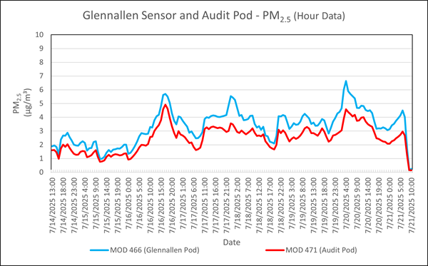
Figure 1 depicts the audit results for the PM2.5 sensor onboard the Glennallen pod, MOD 466. The community pod tracked closely with the audit pod, reporting values within 0-2 µg/m3 above the audit pod’s values.
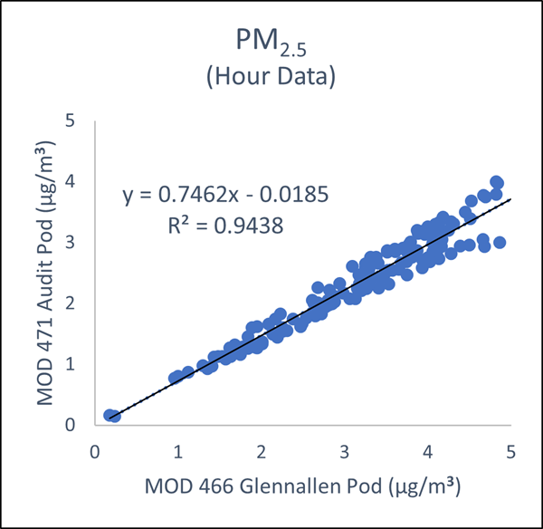
Figure 2 depicts the regression plot results for the PM2.5 sensor audit of the Glennallen pod, MOD 466. The community pod passed the audit with a strong R2 value of 0.9438. The auditing pod was MOD 471.
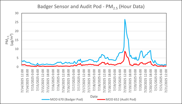
Figure 3 depicts the audit results for the PM2.5 sensor onboard the Badger pod, MOD 670. The community pod tracked closely with the audit pod, reporting values within 0-2 µg/m3 above the audit pod’s values.
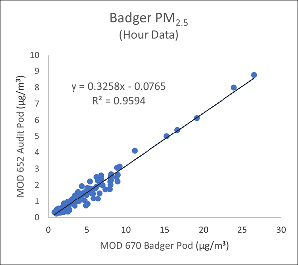
Figure 4 depicts the regression plot results for the PM2.5 sensor audit of the Badger pod, MOD 670. The community pod passed the audit with a strong R2 value of 0.9594. The auditing pod was MOD 652.
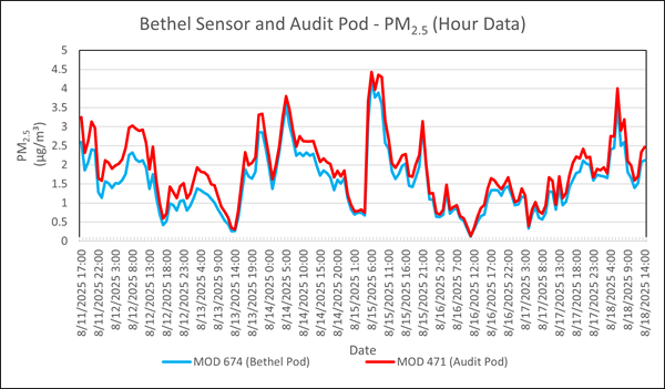
Figure 5 depicts the audit results for the PM2.5 sensor onboard the Bethel pod, MOD 674. The community pod tracked closely with the audit pod, reporting values within 0-1 µg/m3 below the audit pod’s values.
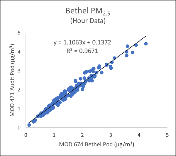
Figure 6 depicts the regression plot results for the PM2.5 sensor audit of the Bethel pod, MOD 674. The community pod passed the audit with a strong R2 value of 0.9671. The auditing pod was MOD 471.
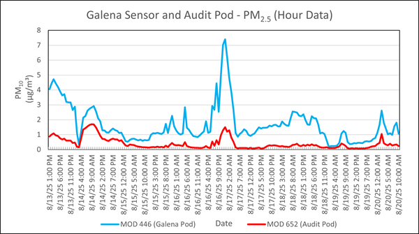
Figure 7 depicts the audit results for the PM2.5 sensor onboard the Galena pod, MOD 446. The community pod produced a similar trendline but reported significantly higher amplitudes than the audit pod.
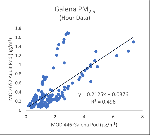
Figure 8 depicts the regression plot results for the PM2.5 sensor audit of the Galena pod, MOD 446. The community pod failed the audit with an R2 value of 0.496. The auditing pod, MOD 652, had performance issues before the Galena deployment and is currently offline for maintenance. The audit will be repeated.
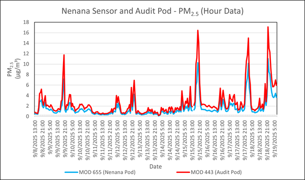
Figure 9 depicts the audit results for the PM2.5 sensor onboard the Nenana pod, MOD 655. The community pod tracked closely with the audit pod, reporting values within 0-1 µg/m3 below the audit pod’s values.
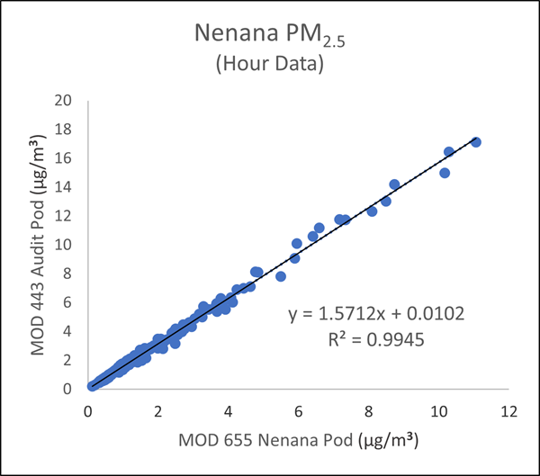
Figure 10 depicts the regression plot results for the PM2.5 sensor audit of the Nenana pod, MOD 655. The community pod passed the audit with a strong R2 value of 0.9945. The auditing pod was MOD 443.
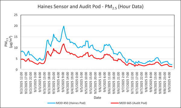
Figure 11 depicts the audit results for the PM2.5 sensor onboard the Haines pod, MOD 450. The community pod tracked decently with the audit pod, reporting values 3-8 µg/m3 above the audit pod’s values.
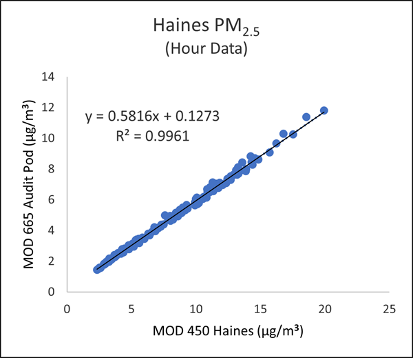
Figure 12 depicts the regression plot results for the PM2.5 sensor audit of the Haines pod, MOD 450. The community pod passed the audit with a strong R2 value of 0.9961. The auditing pod was MOD 665.
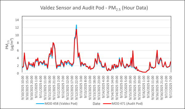
Figure 13 depicts the audit results for the PM2.5 sensor onboard the Valdez pod, MOD 458. The community pod tracked closely with the audit pod, reporting values within 0-2 µg/m3 around the audit pod’s values.
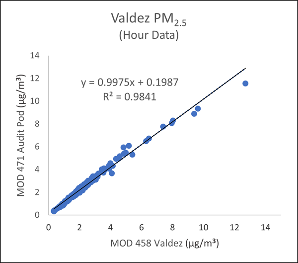
Figure 14 depicts the regression plot results for the PM2.5 sensor audit of the Valdez pod, MOD 458. The community pod passed the audit with a strong R2 value of 0.9841. The auditing pod was MOD 471.
4.3 Data Findings
For data analysis, communities in the sensor network are organized according to general ecoregion. These include the Interior, Western, Southwestern, Southeastern or Panhandle, and Southcentral ecoregions. By grouping sensors into ecoregions, DEC can identify weather and pollution trends affecting one or several ecoregions. Due to the vast size of Alaska, ecoregions may be subdivided into distinct geographic areas; for example, the Southcentral ecoregion can be divided geographically into the Mat-Su Valley area (which includes Anchorage), the Copper River and Chugach Mountain area, and the Kenai Peninsula.
Sensor data can be presented chronologically, to illustrate changes in pollutant concentration over the course of an hour, day, week, month, and year. Time-wise data can be cross-referenced with geographic data to estimate the geospatial movement of air pollution over time and potentially aid in identifying emissions sources. DEC currently uses diurnal and calendar plots to display data in a time-wise manner.
Diurnal plots are useful for comparing changes in pollutant concentration over time in multiple ecoregion (or area within an ecoregion) communities. This facilitates the identification of area- or ecoregion-wide trends in air quality, as well as daily, weekly, or seasonal variation in air quality trends between proximal communities. For example, if pods in an ecoregion show similar PM2.5 patterns over a given time period, that may indicate a single major emission source, such as a large wildland fire. In contrast, differences in PM2.5 patterns among ecoregion communities may indicate multiple distinct, localized emission sources.
Calendar plots are useful diagrams for tracking air quality patterns over long periods of time. Each day is represented by a calendar square; daily average PM2.5 concentrations are calculated and assigned a color code based on the AQI category, where the colors green, yellow, orange, red, purple, and maroon respectively represent “Good”, “Moderate”, “Poor” or “Unhealthy for Sensitive Groups”, “Unhealthy”, “Very Unhealthy”, and “Hazardous” air quality; See Table 3 for a visual representation of the AQI categories. Uncolored calendar squares represent days with <75% data capture. Other incidents may disrupt the sensor’s operation or invalidate its data for one or more days, such as a power outage or a technical issue. By tracking AQI color coding on the calendar plots, DEC can visualize patterns or changes in air quality in specific communities over days, weeks, or months.
| Daily AQI Color | Levels of Concern | Values of Index | Description of Air Quality |
|---|---|---|---|
| Green | Good | 0 to 50 | Air quality is satisfactory, and air pollution poses little or no risk. |
| Yellow | Moderate | 51 to 100 | Air quality is acceptable. However, there may be a risk for some people, particularly those who are unusually sensitive to air pollution. |
| Orange | Unhealthy for Sensitive Groups | 101 to 150 | Members of sensitive groups may experience health effects. The general public is less likely to be affected. |
| Red | Unhealthy | 151 to 200 | Some members of the general public may experience health effects; members of sensitive groups may experience more serious health effects. |
| Purple | Very Unhealthy | 201 to 300 | Health alert: The risk of health effects is increased for everyone. |
| Maroon | Hazardous | 301 and higher | Health warning of emergency conditions: everyone is more likely to be affected. |
The following graphs and figures are all generated with QuantAQ MODULAIRTM data.
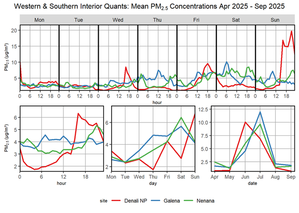
Figure 15 depicts the time series and diurnal graphs of PM2.5 mean concentrations in the Denali NP area and two communities west of Fairbanks, Galena and Nenana, during the reporting period. Communities generally enjoyed low PM2.5 levels, with all communities averaging 5 µg/m3 for the first half of the week, although average PM2.5 levels appeared to rise later in the week, particularly in Denali National Park. This does not reflect average ambient background values on weekends in Denali NP, as the data was impacted by wildland fire smoke. Heavy wildland fire activity throughout the summer produced smoke that affected many Alaska communities. Denali NP experienced three particularly bad air quality days in June and July which skewed the hourly averages between 3 PM and midnight for Wednesday, Friday, and Sundays. Both Nenana and Galena were heavily impacted by wildland fire smoke in early July, which skewed their daily averages for Fridays and Saturdays. All communities demonstrate the impact of seasonal increases in PM2.5 due to wildland fire smoke; PM2.5 levels in April, May, August and September were very low. June and July brought prolonged periods of hot, dry weather, increasing wildland fire activity and smoke impacts in the region.
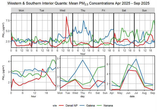
Figure 16 depicts the time series and diurnal graphs of PM2.5 mean concentrations in the Denali NP area, Galena, and Nenana during the reporting period with days affected by wildland fire smoke removed to better illustrate baseline PM2.5 levels. After omission of the heavy wildland fire smoke days, Denali NP sees a drastic reduction in PM2.5 levels, with an average below 3 µg/m3. Removal of wildland fire-affected days also shows that Galena enjoyed good air quality during the weekends.. Nenana had minimal impact from wildland fire smoke, as removal of wildland fire-affected days produced only a minor decrease in reported hourly and daily averages. All communities experienced an increase in average PM2.5 levels in June and July, but after removal of wildland fire-affected days, the reported magnitude of the summer increase is significantly lower.
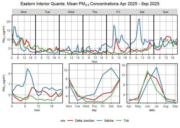
Figure 17 depicts the time series and diurnal graphs of PM2.5 mean concentrations in several eastern Interior region communities; Delta Junction, Salcha, and Tok. There is relatively little difference between Delta Junction and Tok, with both communities showing similar PM2.5 activity across an average day, week and season. Slightly higher levels are seen on Mondays, with levels lowering during the week before gradually increasing towards the weekend. Several large PM2.5 spikes were observed in the averaged hourly data for Fridays and Saturdays, but these paled in comparison to Salcha’s PM2.5 activity. For the most part, the pattern is the same, but Salcha experiences larger magnitudes in its spikes and shifts. Salcha also exhibited the same elevated PM2.5 levels on Monday and PM2.5 spikes on Fridays and Saturdays, but the average values are significantly higher than those seen in Delta Junction and Tok. Over an average week, Salcha sees an earlier and faster rise in PM2.5 levels going towards the weekend, with a higher average ceiling. All communities exhibit significantly higher PM2.5 levels in June and July compared to the spring and fall months, which is almost certainly due to heavy exposure to Interior wildland fire smoke.
Salcha was equipped with an air monitor pod in late May, approximately two months into the reporting period. As a result, the Salcha data is not representative of the entire reporting period.
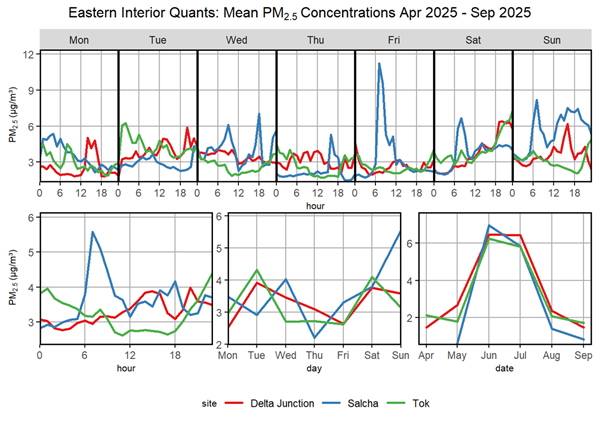
Figure 18 depicts the time series and diurnal graphs of PM2.5 mean concentrations in several eastern Interior region communities with days affected by wildland fire smoke removed to better illustrate baseline PM2.5 levels. After omission of the heavy wildland fire smoke days, changes are seen in the profile of PM2.5 activity in all communities, especially Salcha; hourly averages are reduced, Monday and Saturday averages are halved, and monthly averages in June and July are halved. In Salcha, removal of heavy wildland fire smoke days greatly reduces the daily PM2.5 averages from Thursday through Saturday. The large spike in Salcha’s Monday morning hourly averages is removed, as this was primarily driven by a very smokey Monday in June that reached the ‘Unhealthy’ AQI range, and to a lesser degree, one Monday each in June and July with ‘Moderate’ AQI. Salcha also experienced large PM2.5 spikes on averaged Fridays and Saturdays, which were largely driven by a consecutive Friday and Saturday with ‘Unhealthy’ AQI. Removal of the offending smoke days sees these end-week PM2.5 spikes significantly reduced in magnitude, especially the averaged Saturday spike.
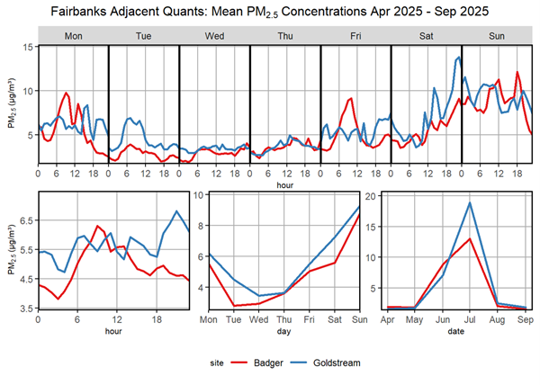
Figure 19 depicts the time series and diurnal graphs of PM2.5 mean concentrations in several communities in the Interior region ; Badger and Goldstream. Both communities displayed similar patterns of PM2.5 activity over a typical week and season, with slight variation seen over an average day. Badger follows a typical pattern where PM2.5 levels rise as people commute to work, peak at around midday, rise again in the afternoon as people commute home from work, and then decrease into the night. Seasonally, both communities enjoyed very low PM2.5 in the spring and fall but were affected by wildland fire smoke during June and July that significantly degraded air quality. Badger experienced an ‘Unhealthy’ AQI day in June and two in July, while Goldstream experienced four ‘Unhealthy’ AQI days in July alone. The worst fire days in both communities were concentrated on Fridays, Saturdays, and Sundays, leading to elevated PM2.5 averages on the weekends.
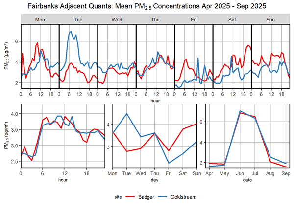
Figure 20 depicts the time series and diurnal graphs of PM2.5 mean concentrations in several Fairbanks-adjacent Interior region communities with days affected by wildland fire smoke removed to better illustrate baseline PM2.5 levels. After omission of the heavy wildland fire smoke days, major changes are seen in the profile of PM2.5 activity in all communities. Baseline PM2.5 levels appear to remain around 2-5 µg/m3 but the magnitude of both PM2.5 spikes and daily, weekly, and monthly averages are reduced. As the worst fire days in both communities happened on Fridays, Saturdays, and Sundays, removing the heavy wildland fire smoke days significantly reduced the hourly and daily averages on the affected days. A PM2.5 spike observed in the Goldstream community’s Tuesday average largely remained after removal of smoke days, suggesting the Tuesday morning surge is the result of other activity. Without wildland fire smoke, Badger experiences a relatively stable pattern of daily averages over the course of a week, with fluctuations largely staying within ±1 µg/m3 of a 3.5 µg/m3 baseline. Goldstream exhibits more variation in PM2.5, with the highest daily average seen on Tuesdays, the lowest seen on Fridays, and middling averages seen at mid-week and on the weekends. With heavy wildland fire days removed, Badger and Goldstream exhibit nearly identical patterns of PM2.5 activity over the season, with very low monthly averages in the spring and fall, and higher monthly averages in the summer, where wildland fire smoke is a recurring problem.
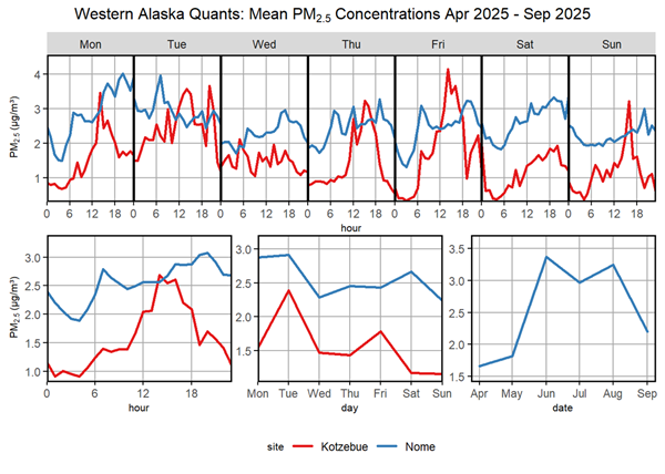
Figure 21 depicts the time series and diurnal graphs of PM2.5 mean concentrations for Kotzebue and Nome, two communities in the Western ecoregion. Both communities enjoyed air quality with hourly, daily, and monthly average PM2.5 levels remaining below 5 µg/m3 throughout the reporting period. Both communities exhibited low levels of PM2.5 in the morning, withlevels gradually rising through an average day before falling back towards baseline in the evenings. Kotzebue’s PM2.5 levels increased and decreased at a faster rate, peaked earlier in the day, and settled at a lower average baseline than PM2.5 levels in Nome. Nome saw characteristic seasonal increases in PM2.5 levels during the summer months, when incidents of dust and wildland fire smoke exposure become more frequent.
On January 18th, the Anchorage-based telecommunications service provider Quintillion Global announced that one of their undersea cables servicing the north slope and northwest communities had been severed by sea ice the day previously. Due to the cable damage, cellular service in the area was affected and the QuantAQ QuantAQ that monitors particulate matter and gaseous pollutants, meteorology is optional.">MODULAIRTM pod in Kotzebue lost contact with both DEC and QuantAQ servers. Due to inclement weather and sea ice, repairs were not possible until the summer. Service was restored at the end of August, and the Kotzebue pod began reporting again at the start of September. Kotzebue’s PM2.5 averages for the current reporting period are based only on data generated in September and is not representative of air quality in Kotzebue during the entire reporting period.
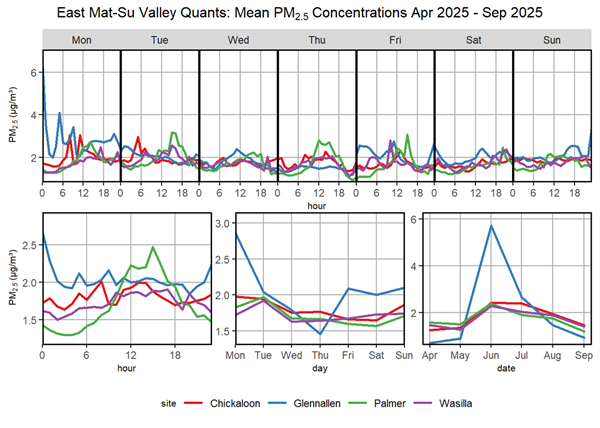
Figure 22 depicts the time series and diurnal graphs of PM2.5 mean concentrations for Chickaloon, Palmer, and Wasilla in the eastern Mat-Su Valley area and Glennallen in the Copper River Valley area. Generally, these communities have ‘Good’ (AQI) air quality, with hourly, daily, and monthly averages for the most part remaining below 5 µg/m3.Overall, the communities showed similar patterns in PM2.5 activity over the interim period, characterized by relatively little variation over the day week and month.
For most of the reporting period, Glennallen enjoyed ‘Good’ (AQI) air quality. However, wildland fire smoke in June raised PM2.5 levels and produced a week with ‘Moderate’ AQI days. Two Mondays in June experienced ‘Moderate’ AQI from smoke exposure in the early morning hours, leading to a slight bump in the midnight to 2 AM hourly averages, the Monday average, and the June average.
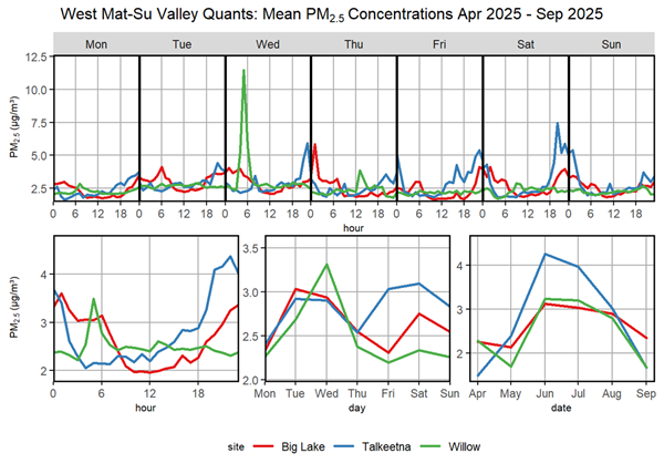
Figure 23 depicts the time series and diurnal graphs of PM2.5 mean concentrations for several southcentral communities in the western Mat-Su Valley area: Big Lake, Talkeetna, and Willow. Generally, these communities have ‘Good’ (AQI) air quality that, for the most part, remains below 5 µg/m3. These communities generally followed a similar pattern in PM2.5 activity over an average day, with low levels at midday and peaks in the mornings and evenings. Over the course of a week, these communities generally showed elevated levels of PM2.5 in the first half of the week, which decreased before rising slightly during the weekend. Willow saw the largest rise in PM2.5 levels in the first half of the week, and Talkeetna saw a dip on Thursdays but otherwise maintained higher PM2.5 levels than the other communities through the latter half of the week. Seasonal patterns are similar across all communities, with Talkeetna seeing the greatest rise in PM2.5 from May to June, and the highest overall PM2.5 levels in June and July by a wide margin.
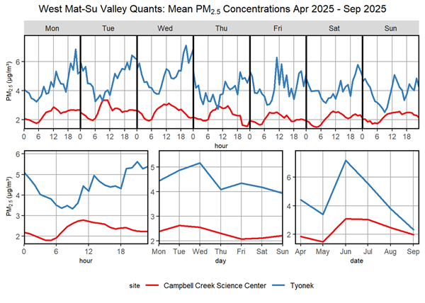
Figure 24 depicts the time series and diurnal graphs of PM2.5 mean concentrations for two southcentral communities in the western Mat-Su Valley area: Anchorage at the Campbell Creek Science Center (CCSC ), and Tyonek. Tyonek is positioned along the coast, directly west from Anchorage across Cook Inlet. The CCSC is located immediately east of Anchorage, between the city and the mountains of Chugach State Park. The communities exhibit approximately similar patterns of PM2.5 activity over an average week and the season, although the magnitude of PM2.5 in Tyonek is generally twice that of PM2.5 at the CCSC . Both communities experienced a slight rise in PM2.5 levels in the first half of the week, which gradually lowered over the latter half of the week. Both communities saw the same seasonal changes in PM2.5 with a dip in May followed by a relative surge in June, with levels tapering off into the fall. In Tyonek, the monthly averages drop at a relatively quick rate, while at CCSC they hold steady for July and drop off slowly, with both communities ultimately reaching below 3 µg/m3 for the September monthly average. The communities showed different daily patterns of PM2.5 with Tyonek showing consistently high variation, with early morning dips followed by a steadily increasing PM2.5 concentration that peaks in the evenings. CCSC experiences a slight rise in PM2.5 levels going into midday, which steadily decreases through the afternoon and evening. Over the reporting period, both sensors recorded very low PM2.5 levels.
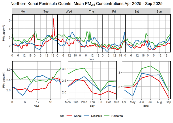
Figure 25 depicts the time series and diurnal graphs of PM2.5 mean concentrations for communities in the western part of the Kenai Peninsula: Kenai, Ninilchik, and Soldotna. For the most part, these communities experienced similar trends in weekly and seasonal PM2.5 activity. Seasonally, the lowest PM2.5 levels were seen in April, May, and September, when the weather is characterized by precipitation and cool temperatures. In the drier, warmer months of June, July, and August dust events and wildland fire smoke exposure is more common, raising PMlevels. Overall PM2.5 levels remained low across the reporting period, with all calculated averages largely remaining below 5 µg/m3.
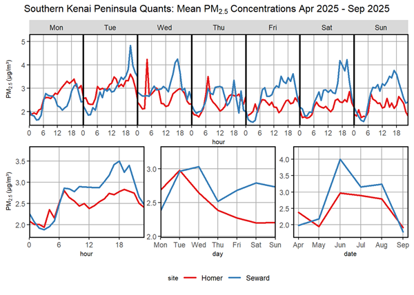
Figure 26 depicts the time series and diurnal graphs of PM2.5 mean concentrations for two communities on the Kenai Peninsula: Homer and Seward. For the most part, these communities experienced similar trends in daily, weekly and seasonal PM2.5 activity. The average day began with low PM2.5 levels, which increased during morning commuting hours, stayed steady throughout midday before rising in the evening, then fell at night. Both communities saw low PM2.5 levels in April, May, and September, with consistently elevated levels across the summer months, though still below 4 µg/m3.
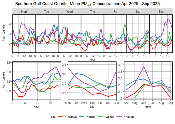
Figure 27 depicts the time series and diurnal graphs of PM2.5 mean concentrations for the southern gulf coast communities of Kodiak, Cordova, Valdez, and Yakutat. All communities generally have ‘Good’ (AQI) air quality, with all averages generally remaining below 5 µg/m3. All communities follow similar patterns of PM2.5 activity across an average day, week, and season. Over the season, all communities saw slight increases in average PM2.5 levels in June. Changes in monthly average PM2.5 level were pronounced in Cordova and Valdez, with very low levels in the spring and fall months and elevated levels in the summer. Kodiak exhibited relatively low variation in monthly averages, while Yakutat saw a rise in PM2.5 levels in June, likely due to the effects of smoke from Interior and Canadian wildland fires.
Due to a roof leak and reconstruction at the host building, the Kodiak pod was taken offline on March 6, 2025, and moved to a secure location. The pod was not repositioned and reconnected until April 8, shortly after the start of the current reporting period.
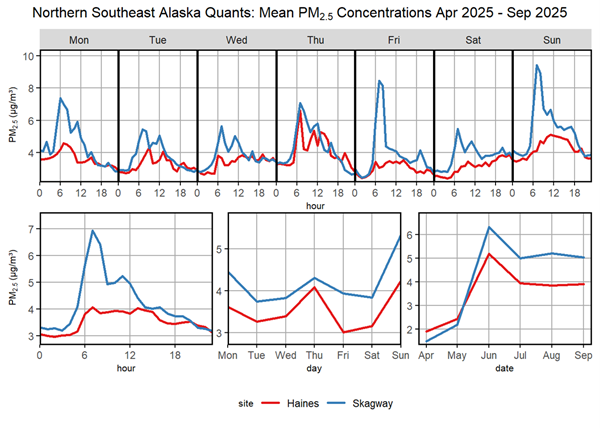
Figure 28 depicts the time series and diurnal graphs of PM2.5 mean concentrations for Haines and Skagway. Daily PM2.5 concentrations are generally similar in both communities, with baseline levels staying below 10 µg/m3. Both communities exhibit similar patterns in PM2.5 activity, with a spike in PM2.5 concentration seen during morning commuting hours, which tapers off over the course of the day. This pattern is consistent across the week in Skagway (with the morning commuting hour PM2.5 spike getting larger on Fridays and Saturdays), but Haines shows a slightly different pattern over the weekend, with a reduction in the morning PM2.5 spike and a relative increase in PM2.5 levels over the afternoon. Over the season, both communities saw a an increase in PM2.5 from May to June, with levels staying elevated for the rest of the reporting period. This PM2.5 activity, particularly in Skagway, is at least partially driven by the activity of tourists activity in the community during the summer tour season.
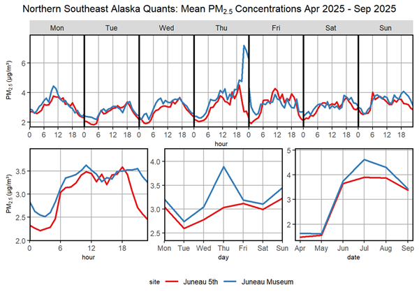
Figure 29 depicts the time series and diurnal graphs of PM2.5 mean concentrations for Juneau at two sites, 5th Street and the Alaska State Museum. Each sensor site represents significantly different geographic conditions, though about a half mile apart. The 5th Street site is located in a neighborhood in the hills in east Juneau, near Starr Hill. The Alaska State Museum site is located near sea level, in downtown Juneau. For the most part, the sensors detect similar PM2.5 levels over time. The Thursday average at the Alaska State Museum is elevated due to a singular event skewing the hourly and daily averages. In Juneau, Independence Day fireworks celebrations take place late at night on July 3rd, which was on a Thursday in 2025. The fireworks are launched near the pier, right above sea level, and are historically detected by the lower-altitude Alaska State Museum pod, but not the higher-altitude 5th Street pod. The smoke and emissions from the fireworks artificially inflated the average PM2.5 values measured by the pod at the State Museum site for the evening hours on Thursdays, the day of Thursday, and the month of July. Generally speaking, outside of holiday celebrations, Juneau enjoys good air quality with baseline PM2.5 levels fluctuating below 5 µg/m3.
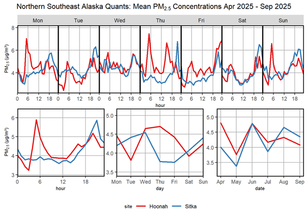
Figure 30 depicts the time series and diurnal graphs of PM2.5 mean concentrations for Hoonah and Sitka, two communities in the northern part of the Southeast ecoregion. Both communities produced different patterns of PM2.5 activity over an average day and over the season. In Hoonah, there is the typical morning PM2.5 spike, but this drops back down to baseline during midday instead of remaining elevated, as is seen in most other communities. Hoonah also sees significant day-to-day variation in hourly average PM2.5 levels. Sitka does not see the typical morning PM2.5 spike but rather sees low PM2.5 levels persist through the morning and for most of the day, before rising in the afternoon and spiking late in the evening. Over the course of a week, Hoonah sees highest daily averages during mid-week and on Mondays, with lower daily averages on Tuesdays and Saturdays. Sitka sees its highest daily averages on Tuesdays and Wednesdays, and lowest daily averages on Thursdays and Fridays. Over the reporting period, both communities enjoyed very low PM2.5 concentrations.
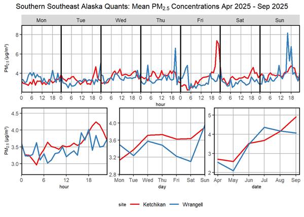
Figure 31 depicts the time series and diurnal graphs of PM2.5 mean concentrations for Ketchikan and Wrangell, two communities near the southern tip of the Southeast ecoregion. Both communities demonstrate similar patterns in PM2.5 activity over an average day, week, and season. PM2.5 activity is generally simple; over an average day, levels rise until peaking in the evening; over an average week, levels rise until peaking on Sundays; over the season, levels rose consistently across the reporting period. Wrangell shows more complex PM2.5 activity; daily patterns are similar to Ketchikan, but with significantly more hour-to-hour fluctuation; weekly and seasonal patterns are similar to Ketchikan but exaggerated, with a steeper drop-off in PM2.5 levels later in the week followed by a shARP rise on Sundays, and a seasonal peak in July. Over the reporting period, both communities enjoyed very low PM2.5 concentrations.

Figure 32 depicts a calendar plot for the Badger area during the reporting period. For the most part, Badger enjoyed ‘Good’ (AQI) air quality throughout the reporting period, except for several weeks in June and July when Interior communities were exposed to large volumes of wildland fire smoke. About halfway through June, Badger was impacted by two sources of smoke that raised baseline PM2.5 levels; fine particulates carried on westerly winds from wildland fires in Canada, and smoke from Interior wildland fires, including the Bear Creek, Twelve Mile Lake, Goldstream, and Monte Cristo fires, among others. Smoke levels peaked on the 22nd, with Badger reporting a maximum hourly average of nearly 160 µg/m3. Light rains at the end of June tamped down on wildland fire smoke across the Interior, but dry conditions returned in early July, bringing more wildland fires. In early July, Badger was impacted by smoke from the Himalaya, Aggie Creek, Goldstream, Monte Cristo, and Bonnifield Creek/Saint George fires, among many others. The Ricks Creek fire produced a particularly large amount of smoke in the area on July 5-6th. Heavy rains tamped down on the wildland fires from July 7-9th, followed by another cycle of dry conditions and wildland fires later in the month. Badger was impacted by smoke from the large Klikhtentotzna fire and several smaller fires on July 12-13th, and from the Monte Cristo fire on the 19th.
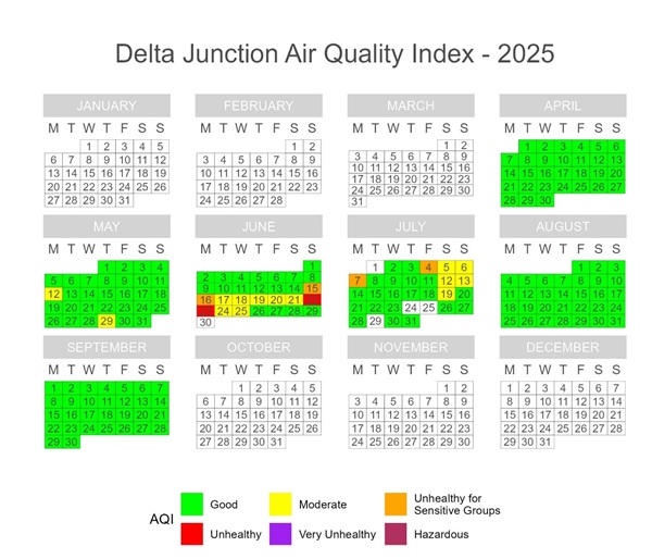
Figure 33 depicts a calendar plot for the community of Delta Junction during the reporting period. Delta Junction generally had ‘Good’ (AQI) air quality throughout the reporting period, except for several weeks when Interior communities were exposed to large volumes of wildland fire smoke tempered by cycles of rainfall. About halfway through June, Delta Junction was impacted by two sources of smoke that raised baseline PM2.5 levels; fine particulates carried on westerly winds from wildland fires in Canada, and smoke from Interior wildland fires, including the Bear Creek, Twelve Mile Lake, and Monte Cristo fires. Smoke levels peaked on June 23rd, with Delta Junction reporting a maximum hourly average exceeding 130 µg/m3. In early July, Delta Junction was impacted by smoke from the Bonanza Creek, Bonnifield Creek/Saint George and Dry Creek fires, and later, from the Sand Lake and Twelve Mile Lake fires. Delta Junction was impacted by smoke from the large Klikhtentotzna fire and several smaller fires on July 12-13th, and from the Monte Cristo fire on the 19th.
The pod began experiencing disruptions to its PM sensor activity in late June, characterized by frequent outages which affected data collection. The issue persisted through July before resolving.
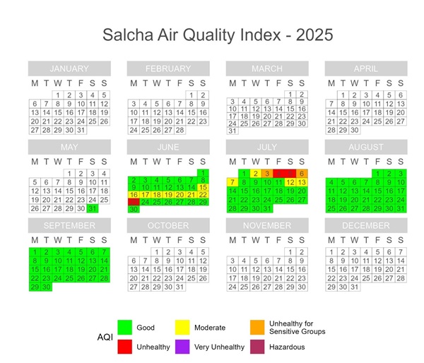
Figure 34 depicts a calendar plot for the community of Salcha during the reporting period. Salcha was equipped with an air monitoring pod on May 30th, so there is no data for the first two months of the reporting period. Salcha generally had ‘Good’ (AQI) air quality throughout the reporting period, except for several weeks when Interior communities were exposed to large volumes of wildland fire smoke tempered by cycles of rainfall. About halfway through June, Salcha was impacted by two sources of smoke that raised baseline PM2.5 levels; fine particulates carried on westerly winds from wildland fires in Canada, and smoke from Interior wildland fires, including the Bear Creek, Twelve Mile Lake, and Monte Cristo fires. Smoke levels peaked early on June 23rd, with Salcha reporting a maximum hourly average exceeding 225 µg/m3. In early July, Salcha was impacted by smoke from the Bonanza Creek, Bonnifield Creek / Saint George and Dry Creek fires, and later, from the Sand Lake and Twelve Mile Lake fires. Salcha was impacted by smoke from the large Klikhtentotzna fire and several smaller fires on July 12-13th.
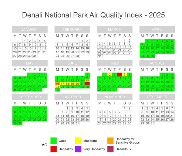
Figure 35 depicts a calendar plot for the Denali NP pod during the reporting period. Denali NP enjoyed air quality in the ‘Good’ AQI range for almost the entire reporting period, except for a few weeks in June and early July when Interior wildland fire activity was high. About halfway through June, Denali NP was impacted by fine particulates carried on westerly winds from wildland fires in Canada. PM2.5 levels peaked late on June 22nd due to the proximal Bear Creek fire, with Denali NP reporting a maximum hourly average exceeding 438 µg/m3. In early July, Denali NP experienced several pulses of smoke from more distant Interior wildland fires. An afternoon PM2.5 surge on July 2nd was probably caused by smoke from the carried on winds southwest from the Ninety Eight fire, and to a lesser degree the Nenan Ridge, Bonanza Creek, Goldstream, and Aggie Creek fires. A larger surge on July 4th peaked at almost 200 µg/m3 and persisted with elevated PM2.5 levels through the 5th before returning to baseline. This last PM2.5 surge was likely caused by smoke from multiple northern and eastern Interior wildland fires being mixed and carried east/southeast by the wind.
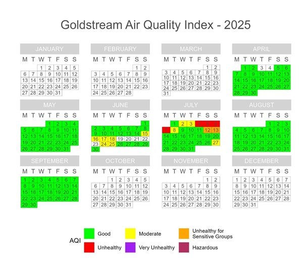
Figure 36 depicts a calendar plot for the Goldstream area during the reporting period. For the most part, Goldstream enjoyed ‘Good’ (AQI) air quality throughout the reporting period, except for several weeks in June and July when Interior communities were exposed to large volumes of wildland fire smoke tempered by cycles of rainfall. About halfway through June, Goldstream was impacted by two sources of smoke that raised baseline PM2.5 levels; fine particulates carried on westerly winds from wildland fires in Canada, and smoke from Interior wildland fires, including the Bear Creek, Twelve Mile Lake, Goldstream, and Monte Cristo fires. The outlet powering the air monitor reset on June 19th, shutting down the pod until the outlet was re-activated on the 23rd and causing a failure to capture some of the worst smoke days in June. Early July saw a resurgence of wildland fires around Fairbanks, which had a significant impact on the Goldstream area. The Aggie Creek, Goldstream, Nenana Ridge, Bonanza Creek, and Ninety Eight fires produced smoke that swept over Goldstream in the first few days of July, followed by a large influx of smoke from the Ricks Creek fire on July 5-6th that saw PM2.5 levels peak at nearly 200 µg/m3. Goldstream was impacted by smoke from the Klikhtentotzna fire and several smaller fires on July 12-13th.
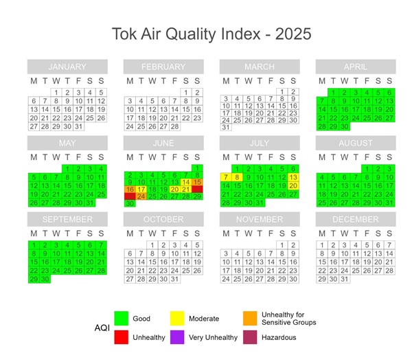
Figure 37 depicts a calendar plot for the community of Tok during the reporting period. Tok generally had ‘Good’ (AQI) air quality throughout the reporting period, except for a few multi-day periods when Interior communities were exposed to large volumes of wildland fire smoke tempered by cycles of rainfall. About halfway through June, Tok was impacted by fine particulates carried on westerly winds from wildland fires in Canada. Several days later, Tok was affected by smoke from emergent Interior wildland fires, including the Sand Lake, Twelve Mile Lake, River Trail, Ridgeline, and Kechumstuk Creek fires. Smoke levels peaked on the night of June 23rd, with Tok reporting a maximum hourly average of almost 145 µg/m3. In July, changes in wind direction brought a mixture of smoke from Canadian and Interior Alaska wildland fires that affected Tok on the 7-8th, with peak hourly average PM2.5 levels exceeding 70 µg/m3. July 13th saw mostly smoke from Canadian wildland fires, and July 20th saw mostly smoke from Interior Alaska wildland fires, but no smoke day in July exceeded the ‘Moderate’ AQI range.
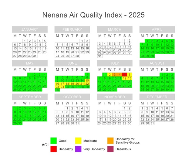
Figure 38 depicts a calendar plot for the community of Nenana during the reporting period. Nenana enjoyed air quality in the ‘Good’ AQI range for almost the entire reporting period, except for a few weeks in June and early July when Interior wildland fire activity was high. About halfway through June, Nenana was impacted by smoke from wildland fires in Canada, moderately increasing PM2.5 levels. Several days later, Nenana started to feel smoke from numerous Interior Alaska wildland fires, including the Nenana Ridge, Goldstream, Bonanza Creek, Saint George Creek / Bonnifield Creek, and Bear Creek fires. June 20-22nd saw a series of mid-morning PM2.5 spikes that exceeded 43, 72, and 59 µg/m3, respectively. These fires were tamped down by rain at the end of the month, but subsequent hot, dry conditions lead to their resurgence in early July. The same cluster of Interior wildland fires pummeled Nenana with smoke in the first week of July; July 4th saw a midday spike exceeding 125 µg/m3, while July 5th had higher overall levels including a morning and afternoon spike each exceeding 100 µg/m3. Nenana may have also been affected on the 5th and 6th by smoke from the Ricks Creek, Ninety Eight, and Monte Cristo fires being blown west across Fairbanks. On the 12th and 13th, Nenana was moderately affected by smoke from the distant Klikhtentotzna fire and it’s smaller satellite fires.
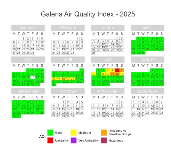
Figure 39 depicts a calendar plot for the community of Galena during the reporting period. Galena enjoyed air quality in the ‘Good’ AQI range for almost the entire reporting period, except for a few weeks in June and early July when Interior wildland fire activity was high. About halfway through June, Galena was impacted by smoke from numerous small regional fires, including the Nikolai, Kola, Gisasa, and Teethcanoe fire, leading to five days of ‘Moderate’ (AQI) air quality. In July, Galena was impacted by smoke from wildland fires across the state. The first week of July saw multiple wildland fires in the area surrounding Fairbanks produce smoke that was carried west on the wind into Galena. This smoke influx elevated baseline PM2.5 levels and produced a spike of PM2.5 on July 5th that saw a peak hourly average exceeding 170 µg/m3. Rains tamped down on the Interior wildland fires, leading to a brief respite from the smoke. In the second week of July, Galena was affected by smoke from regional wildland fires, including the Klikhtentotzna fire and the smaller Anguitakada, Wheeler, Caribou, Richards, and Moldy fires. This smoke event pushed Galena’s AQI into the ‘Unhealthy for Sensitive Groups’ range for two days and saw a peak PM2.5 hourly average midday on the 11th with PM2.5 levels exceeding 95 µg/m3.
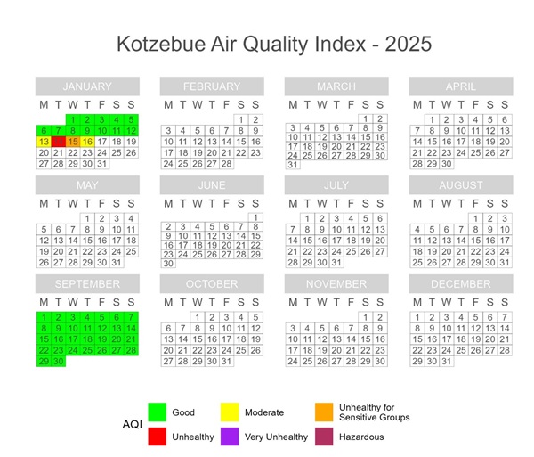
Figure 40 depicts a calendar plot for the community of Kotzebue during the reporting period. The pod went offline on the morning of January 17th due to a severed subsea cable off the western coast of Alaska. Quintillion’s network hosts several internet and cellular providers, including AT&T (which the QuantAQ MODULAIRTM pods use to transmit data), which all saw disruptions to their service due to the cable break. The Kotzebue pod was brought back online at the beginning of September and reported air quality in the ‘Good’ AQI range for the remainder of the reporting period.

Figure 41 depicts a calendar plot for the community of Nome during the reporting period. For the most part, Nome enjoyed air quality in the ‘Good’ AQI range, with a few days reaching the ‘Moderate’ AQI range.
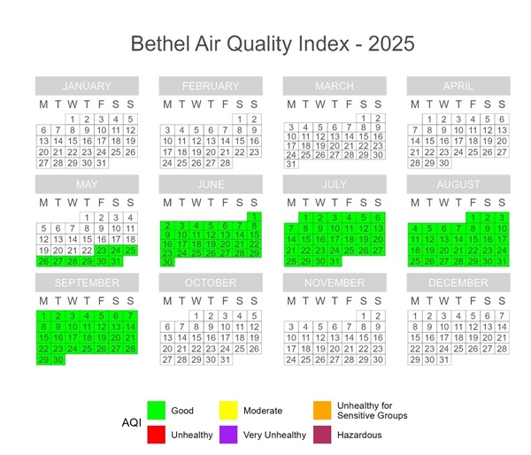
Figure 42 depicts a calendar plot for the community of Bethel during the reporting period. During the previous reporting period, Bethel experienced significant issues with cellular connectivity. The original pods installed in the community were unable to make a connection and were taken down on January 29. The Bethel community went without an air monitor pod for several months until QuantAQ 674 was installed on May 22, part way into the current reporting period. For the rest of the reporting period, Bethel enjoyed air quality in the ‘Good’ AQI range.
The Bethel pod received a gaseous model update on August 29th.
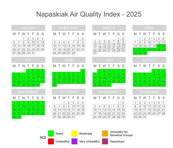
Figure 43 depicts a calendar plot for the community of Napaskiak during the reporting period. During the previous reporting period, Napaskiak experienced significant issues with cellular connectivity. QuantAQ 442 remained in Napaskiak while DEC attempted to troubleshoot the connectivity problem. The pod regained connectivity and data collection resumed mid-April. The pod measured ‘Good’ (AQI) air quality for the rest of the reporting period.
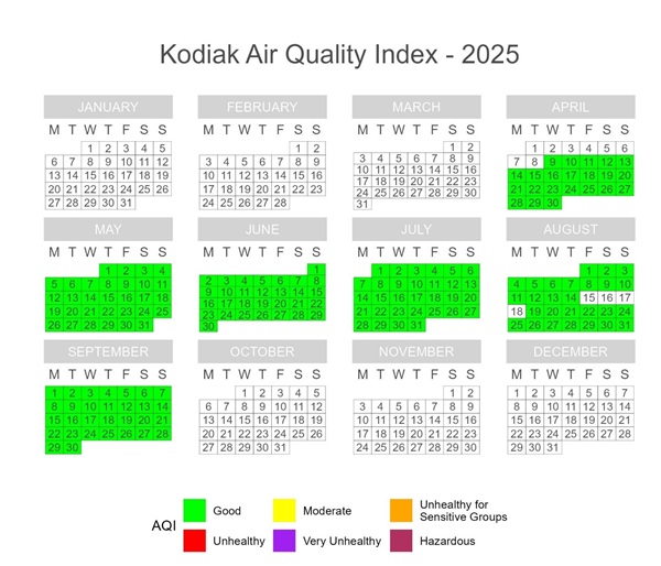
Figure 44 depicts a calendar plot for the island-based community of Kodiak during the reporting period. Kodiak generally enjoys air quality in the ‘Good’ AQI range. Aside from days with no data, the Kodiak pod reporting ‘Good’ (AQI) air quality throughout the reporting period.
Due to a roof leak and construction at the host building, the Kodiak pod was taken offline on March 6th, 2025, and moved to a secure location. The pod was not reconnected until April 8th, 2025, about one week into the current reporting period. The pod was offline for several days in mid-August due to a power supply issue at the hosting facility.

Figure 45 depicts a calendar plot for the community of Big Lake during the reporting period. Big Lake enjoyed ‘Good’ (AQI) air quality for most of the reporting period, although there was one day with air quality in the ‘Moderate’ AQI range. This was a warm day with no rain or fog, which saw PM2.5 levels rise slowly over the day and peak in the evening; the daily AQI average tipped into the ‘Moderate’ range, but there was no significant surge or spike in PM2.5 concentration. Smoke from the Bear Creek fire approximately 38 miles north of Denali National Park may have contributed to these elevated PM2.5 levels in Big Lake.
In mid-September, the pod’s power cord was accidentally unplugged over the weekend. The power cord was plugged back in the following Monday, and connectivity was restored.
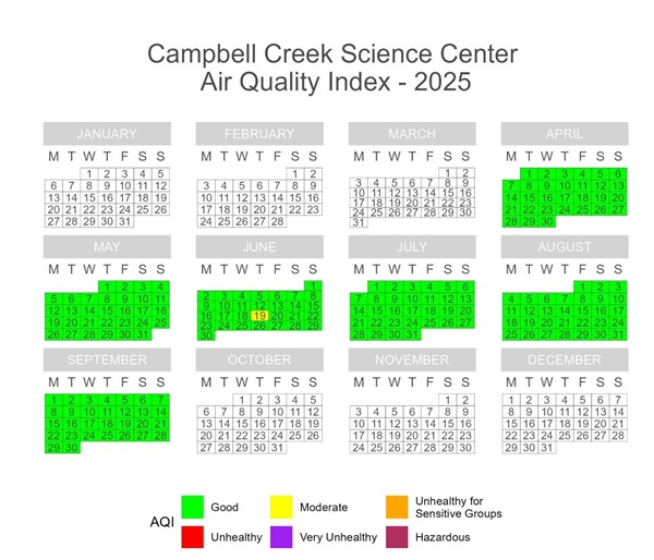
Figure 46 depicts a calendar plot for the Campbell Creek Science Center located in east Anchorage during the reporting period. The Campbell Creek Science Center pod experienced air quality in the ‘Good’ AQI range for almost the entire reporting period, except for June 19th, where the air quality reached the ‘Moderate’ AQI range.

Figure 47 depicts a calendar plot for the community of Chickaloon/Sutton-Alpine during the reporting period. The air sensor is located closer to the community of Sutton-Alpine but is located at a building whose mailing address corresponds to the community of Chickaloon. Chickaloon/Sutton-Alpine enjoyed air quality in the ‘Good’ AQI range for the entire reporting period.

Figure 48 depicts a calendar plot for the community of Talkeetna during the reporting period. The Talkeetna pod measured air quality in the ‘Good’ AQI range for almost the entire duration of the reporting period. During a three-day period in mid-June, Talkeetna saw air quality enter the ‘Moderate’ AQI range. The pod reported a series of brief PM2.5 spikes late in the evening on the 18th and 19th, and in the mid-morning on the 19th and 20th. Baseline PM2.5 levels were moderately elevated on the 19th.

Figure 49 depicts a calendar plot for the community of Palmer during the reporting period. Palmer had air quality in the ‘Good’ AQI range for the entirety of the reporting period.

Figure 50 depicts a calendar plot for the community of Wasilla during the reporting period. Wasilla had air quality in the ‘Good’ AQI range for the entirety of the reporting period.

Figure 51 depicts a calendar plot for the community of Willow during the reporting period. Willow generally enjoyed ‘Good’ (AQI) air quality through the reporting period, with occasional days in the ‘Moderate’ AQI range.

Figure 52 depicts a calendar plot for the community of Tyonek during the reporting period. Tyonek generally has ‘Good’ (AQI) air quality, but sometimes ‘Moderate’ (AQI) air quality, particularly during dry weather. Brief but sizeable spikes in PM2.5 concentration were seen throughout the beginning of April, leading to the ‘Moderate’ (AQI) air level on April 2nd. Background levels were slightly raised on April 16th, pushing the daily average into the ‘Moderate’ AQI range despite a lack of pronounced PM2.5 spikes. In mid-June, wildland fires in Canada produced smoke that was blown westward into Alaska, creating daytime increases in PM2.5 concentration that pushed the daily AQI into the ‘Moderate’ range on June 13-14th, 16th, and 18-20th. Daytime PM2.5 levels continued to fluctuate above baseline, producing additional ‘Moderate’ AQI days on June 30th, July 5th, and July 9th.
The Tyonek pod has a power cord that runs through a wall port to connect to an indoor power outlet. On June 11th, staff at the hosting facility were re-arranging furniture and accidentally unplugged the pod’s power cord. The pod was plugged back in and resumed operation on June 12th.
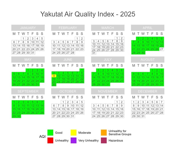
Figure 53 depicts a calendar plot for the community of Yakutat during the reporting period. Yakutat generally enjoyed ‘Good’ (AQI) air quality through the reporting period, with one day in the ‘Moderate’ AQI range. The second week of June saw a minor increase in background PM2.5 levels that lasted several days. A modest early morning spike in PM2.5 was seen on June 9th. Together, this PM2.5 activity pushed the AQI for June 9th into the ‘Moderate’ range.

Figure 54 depicts a calendar plot for the community of Cordova during the reporting period. Cordova had air quality in the ‘Good’ AQI range for the entirety of the reporting period.
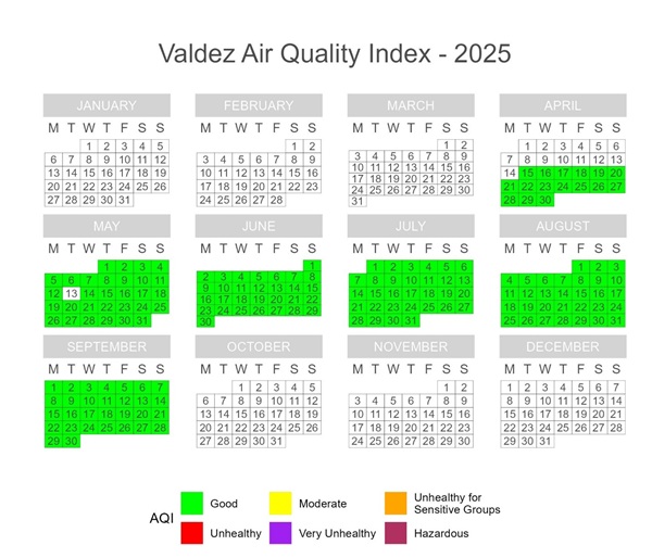
Figure 55 depicts a calendar plot for the community of Valdez during the reporting period. Valdez had air quality in the ‘Good’ AQI range for all days there was a pod installed and operational during the reporting period.
Valdez was initially equipped with the QuantAQ 666 pod on April 14th, which exhibited a multitude of persistent performance issues until it was replaced by QuantAQ 458 on May 13th.
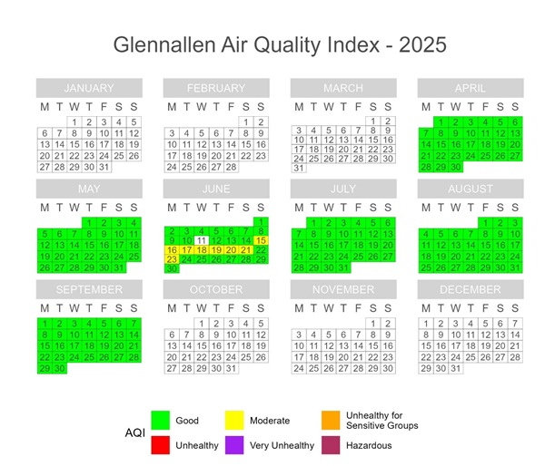
Figure 56 depicts a calendar plot for the community of Glennallen during the reporting period. For the most part, Glennallen enjoys ‘Good’ (AQI) air quality. A stretch of ‘Moderate’ AQI days were observed in mid-June. Initially, the increased PM2.5 levels were linked with an influx of smoke from Canadian wildland fires. Later in the month, the East Gakona River and Fish Lake fires began burning in close proximity to Glennallen, likely contributing to a large PM2.5 spike observed early in the morning on June 23rd, where the midnight hourly average almost reached 110 µg/m3. Glennallen saw ‘Good’ (AQI) air quality for the remainder of the reporting period.

Figure 57 depicts a calendar plot for the community of Homer during the reporting period. Homer had air quality in the ‘Good’ AQI range for almost the entirety of the reporting period, with one day reaching the ‘Moderate’ AQI range. On April 2nd, a brief spike in PM2.5 was reported early in the morning, with the 4 AM hourly average exceeding 55 µg/m3 before returning to baseline. This PM2.5 spike coincided with a spike in PM10 and CO, suggesting a source of combustion was near the pod, such as a large idling vehicle.
Homer experienced storm weather from August 27-28th that disrupted power supply to the pod. Power was restored around midday on the 28th, which meant there was insufficient data to calculate a daily average.
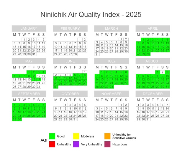
Figure 58 depicts a calendar plot for the community of Ninilchik during the reporting period. The Ninilchik pod measured ‘Good’ (AQI) air quality for the entire duration of the reporting period, except for several days where there was insufficient data to calculate a daily average.
In mid-May, the pod was found unplugged, possibly due to vandalism. Although the pod was eventually plugged back in, the time spent unplugged may have exposed it to water. The pod continued to experience power supply issues for the next several weeks, until it was discovered that water damage had rusted the power block. The damaged components were replaced, and the pod was returned to full operation by the evening of June 5th and generated enough data to calculate daily averages again from June 6th.

Figure 59 depicts a calendar plot for the community of Kenai during the reporting period. The Kenai pod measured ‘Good’ (AQI) air quality for the entire duration of the reporting period.

Figure 60 depicts a calendar plot for the community of Seward during the reporting period. Seward enjoyed ‘Good’ (AQI) air quality for almost the entirety of the reporting period, except for one ‘Moderate’ AQI day.

Figure 61 depicts a calendar plot for the community of Soldotna during the reporting period. Soldotna enjoyed ‘Good’ (AQI) air quality for almost the entirety of the reporting period, except for one ‘Moderate’ AQI day.
The Soldotna pod received a gaseous model update on August 29th.

Figure 62 depicts a calendar plot for the community of Haines during the reporting period. For most of the reporting period, Haines had ‘Good’ (AQI) air quality, with a handful of days experiencing air quality in the ‘Moderate’ AQI range. On May 8, Haines experienced a coincident surge in PM2.5, PM10, and CO that lasted through the workday, possibly as a result of one or more nearby idling vehicles. In mid-June, smoke from Canadian wildland fires was blown west, with some settling in the panhandle region and increasing local PM2.5 levels around the 15th and 16th. Smoke from dozens of small fires across eastern Alaska was being blown east and southeast into the panhandle, increasing baseline PM2.5 levels again from June 21st - 23rd. These later incidents also saw an increase in PM10 and CO that was not seen on the 15th and 16th. In early September, smoke from Canadian wildland fires in British Colombia passed over the Coastal Barrier Mountains and raised PM2.5 levels in Haines on September 4th and 5th.
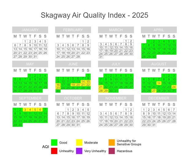
Figure 63 depicts a calendar plot for the community of Skagway during the reporting period. For most of the reporting period, Skagway had ‘Good’ (AQI) air quality, with a handful of days in the ‘Moderate’ AQI range. In mid-June, smoke from Canadian wildland fires was blown west, with some settling in the panhandle region and increasing local PM2.5 levels from the 14th to the 16th. Smoke from dozens of small fires across eastern Alaska was blown east and southeast into the panhandle, increasing baseline PM2.5 levels from June 19th - 23rd. In early September, smoke from Canadian wildland fires in British Colombia passed over the Coastal Barrier Mountains and raised PM2.5 levels in Skagway from September 3rd through the 6th.
Skagway is a busy tourist destination in the summer. Multiple cruise ships dock in Skagway and idle in port as tourists visit the town. Tourist activity produces substantial emissions in the form of dust and vehicle exhaust.

Figure 64 depicts a calendar plot for the 5th Street site pod in Juneau during the reporting period. The pod in Juneau at 5th Street measured air quality in the ‘Good’ AQI range for most of the reporting period, with a small number of ‘Moderate’ AQI days. In mid-June, many wildland fires were burning in Interior Alaska and the Yukon Territory in Canada. Shifting wind patterns brought smoke down towards the panhandle and raised PM2.5 levels in Juneau at 5th Street on the 21st and 22nd. In early September, a series of large forest fires began burning in British Columbia, Canada, and wind carried this smoke into the panhandle, raising PM2.5 levels in Juneau at 5th Street on the 4th and 5th.
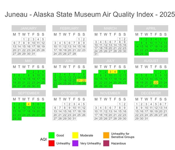
Figure 65 depicts a calendar plot for the State Museum site pod in Juneau during the reporting period. The pod in Juneau at the State Museum measured air quality in the ‘Good’ AQI range for most of the reporting period, with a small number of ‘Moderate’ AQI days. In mid-June, many wildland fires were burning in Interior Alaska and the Yukon Territory in Canada. Shifting wind patterns brought smoke down towards the panhandle and raised PM2.5 levels in Juneau at 5th Street on the 21st and 22nd. Juneau celebrates 4th of July beginning with a fireworks display on July 3rd, which is picked up by the sensor at the State Museum. In early September, a series of large forest fires began burning in British Columbia, Canada, and wind carried this smoke into the panhandle, raising PM2.5 levels in Juneau at 5th Street on September 4th.

Figure 66 depicts a calendar plot for the community of Hoonah during the reporting period. Most days enjoyed air quality in the ‘Good’ AQI range, although air quality occasionally entered the ‘Moderate’ AQI range. The ‘Moderate’ AQI days in early April were caused by slightly larger-than-average PM2.5 spikes during morning and afternoon commuter hours. June 21st saw a large PM2.5 spike in the morning, simultaneous with a small spike in CO, which could plausibly be caused by a large vehicle idling near the sensor. Similarly, July 28th had slightly elevated baseline PM2.5 levels but was pushed into the ‘Moderate’ AQI range because of a large PM2.5 spike exceeding 50 µg/m3 during afternoon hours.
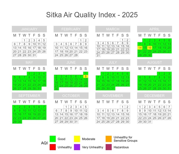
Figure 67 depicts a calendar plot for the community of Sitka during the reporting period. For most of the reporting period, Sitka had ‘Good’ (AQI) air quality, with the rare day in the ‘Moderate’ AQI range. All days with a ‘Moderate’ (AQI) air quality were characterized by cool temperatures, overcast skies, and light to moderate precipitation with wind.

Figure 68 depicts a calendar plot for the community of Ketchikan during the reporting period. For most of the reporting period, Ketchikan had ‘Good’ (AQI) air quality with the exception of a few days that reached the ‘Moderate’ AQI range. July 4th saw normal PM2.5 levels throughout the day, until a sudden spike in the evening peaked at almost 80 µg/m3 and pushed the daily AQI into the ‘Moderate’ range. The PM2.5 spike can likely be attributed to July 4th fireworks celebrations.
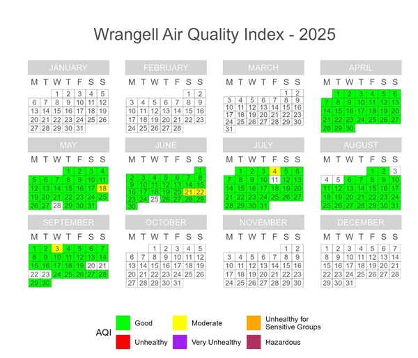
Figure 69 depicts a calendar plot for the community of Wrangell during the reporting period. For most of the reporting period, Wrangell had ‘Good’ (AQI) air quality, with some days in the ‘Moderate’ AQI range. July 3rd and 4th saw normal PM2.5 levels throughout the day, although several increasingly large spikes were seen late at night on the 3rd going into the 4th. The PM2.5 spike on July 4th can likely be attributed to fireworks celebrations.
The Wrangell pod has experienced several periods of data disruption due to malfunctions with the PM sensor. DEC is currently troubleshooting the situation. The outage in early August was caused by the power cable being unplugged.
5 Future Plans
By the end of the reporting period, DEC has deployed a majority of its QuantAQ MODULAIRTM sensors in communities throughout Alaska. DEC will continue to monitor the pod data feeds to identify erroneous data and hardware issues and will continue working on data analysis and providing meaningful insights and outreach material to participating communities and the public. DEC has continued to track pod performance with the goal of developing a robust, multi-year data set that will enable the observation of seasonal trends and season-associated degradation in performance and data quality. To address network limitations that prevent servicing communities that have limited cellular coverage, DEC is working on procuring Wi-Fi enabled sensors that to expand the sensor network into areas previously limited by lack of cellular coverage.
Community outreach remains an integral pillar of the low-cost air sensor network. DEC has continued to update its publicly accessible AQI website, host quarterly community engagement calls, and provide winter/summer data reports to interested communities. DEC hopes to gain feedback from participating communities and tribal entities in order to provide meaningful data products and analysis and improve community outreach. The next interim report will include data from communities participating in the network between October 1st, 2025, and March 31st, 2026.
6 References
-
World Health Organization, Air Pollution, https://www.who.int/health-topics/air-pollution. Accessed December 16, 2025.
-
Nelson et al., Environmental Health Consults in Children Hospitalized with Respiratory Infections. April 2021.
-
Alaska Department of Environmental Conservation, Quality Assurance Project Plan, Community-Based Air Sensor Network. December 2023.
-
Alaska Department of Environmental Conservation, Alaska Community Air Sensor Network, 1st Interim Report. December 2024. https://dec.alaska.gov/air/air-monitoring/instruments-sites/community-based-monitoring/interim-reports/.
 Indicates an external site.